Playing the Beer Game Using Reinforcement Learning

The Classical Beer Game

The beer game is a widely used in-class game that is played in supply chain management classes to demonstrate a phenomenon known as the bullwhip effect. The game consists of a serial supply chain network with four players—a retailer, a wholesaler, a distributor, and a manufacturer.

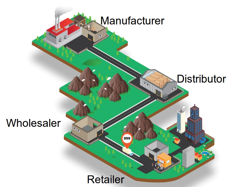
In each period of the game, the retailer experiences a random demand from customers. Then the four players each decide how much inventory of "beer" to order. The retailer orders from the wholesaler, the wholesaler orders from the distributor, the distributor from the manufacturer, and the manufacturer orders from an external supplier that is not a player in the game. If a player does not have sufficient inventory to serve the current period's demand (or orders), the unmet demands are backordered; that is, the customer or downstream node waits until inventory is available. The manufacturer's supplier, however, never has shortages—it is assumed to have infinite supply. There are deterministic transportation and information lead times, though the total lead time is stochastic due to stockouts at upstream nodes. Each player may have nonzero shortage and holding costs.

The players' goal is to minimize the total holding and shortage costs of the whole supply chain. This is therefore a cooperative game, but the players are not allowed to communicate with one another, and moreover they do not know the inventory levels or ordering decisions at the other players—each player only has access to local information.

The beer game has been written about quite a bit in the academic literature. Most of this research asks, how do human players play the beer game? and examines the bullwhip effect and other phenomena that arise from this play. An important question that has not been addressed much in the literature is, how should players play the beer game? In other words, what is the optimal inventory policy that a given player should follow? This is a difficult question, especially when the other players do not, themselves, follow an optimal policy. (The beer game can be classified as a multi-agent, cooperative, decentralized, partially observed Markov decision process, a class of problems that is known to be NEXP-complete—that is, very hard.)

Answering the question of how players should play will have implications not only for the beer game, but also for optimizing inventory decisions in supply chains more generally.

The Machine Learning Model

Our research addresses this question by developing a machine learning (ML) or artificial intelligence (AI) agent to play the beer game.

We propose a modified Deep Q-Network (DQN) to solve to this problem. DQN has been used to solve single-agent games (such as Atari games) and two-agent zero-sum games (such as Go). However, the beer game is a cooperative, non-zero-sum game. Therefore, using DQN directly would result in each player minimizing its own cost, ignoring the system-wide cost. To fix this issue, we propose a feedback scheme that causes the agents to learn to minimize the whole cost of system. In particular, we update the observed reward of each agent i in each period t using

in which we penalize the agent using the sum of the costs of the other agents. Therefore, the agents learn to minimize the total cost of the system instead of just their own costs.

How Well Does It Play the Game?

We present the results from a straightforward version of the game in which the DQN plays the role of the wholesaler and the other three players each follow a base-stock policy. (A base-stock policy means we always order to bring the inventory position—on-hand inventory minus backorders plus on-order inventory—equal to a fixed value, called the base-stock level. A base-stock policy is known to be optimal for the beer game, assuming all four players use it.) Each stage has a holding cost of $2 per item per period. The retailer has a shortage cost of $2 per item per period and the other stages do not have a shortage cost. The customer demand is either 0, 1, or 2 in each time period. (If these numbers seem small to you, think of them as cases or truckloads.) And, here is the way that the wholesaler learns:

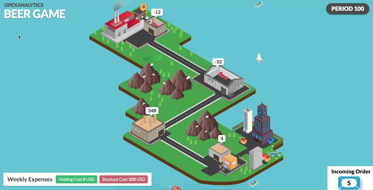
Before the algorithm is trained, the wholesaler plays pretty badly. It stocks way too much inventory, as you can see in the figure below, and causes stockouts at the upstream stages. (Positive inventory is shown as brown boxes and positive numbers. Backorders are shown as red boxes and negative numbers.)

After 1000 training episodes, the DQN agent has learned that there is positive holding cost and so it is better to keep its inventory level smaller.

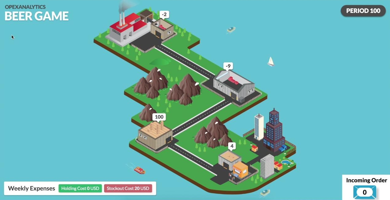
After 2000 training episodes, it has learned that there is no stock-out cost upstream from the retailer, so it is better to keep its inventory level negative. In general, the whole network is more stable and the inventory levels are all closer to zero than in the previous screenshots.

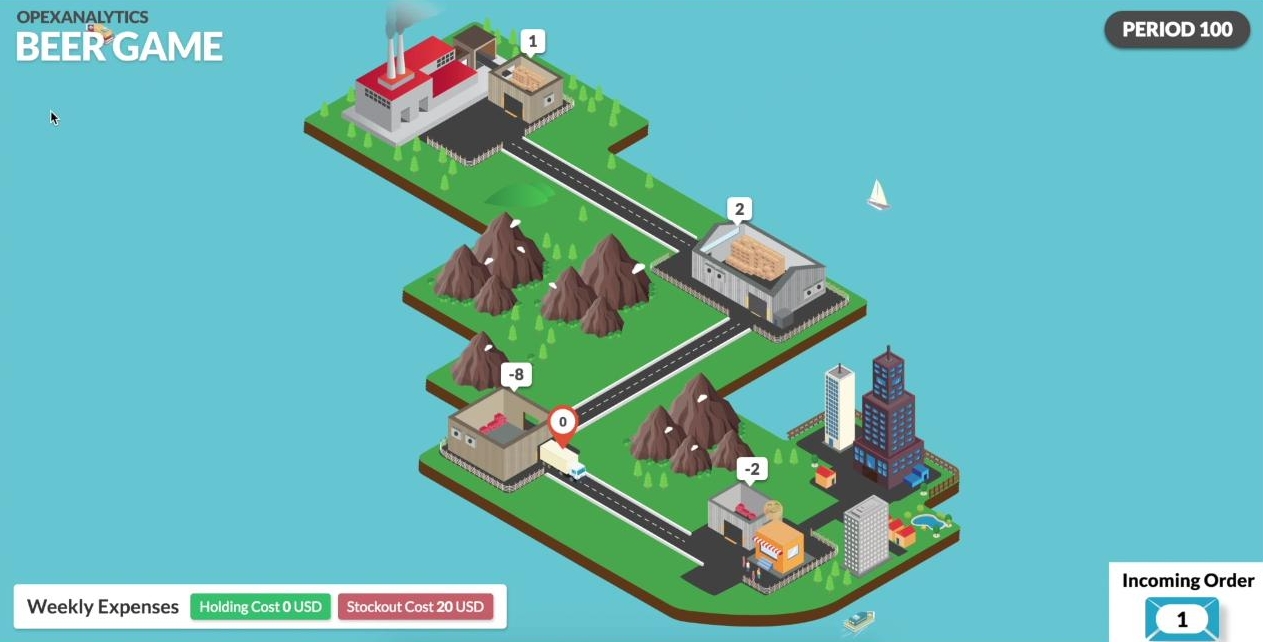
After 45000 training episodes, the AI agent not only plays in a way to keep its inventory level and cost close to zero, but also to minimize the total cost of the system. In fact, it plays very close to a base-stock policy, which is the optimal policy. The whole network is more stable and the inventory levels are closer to zero than in previous screenshots.

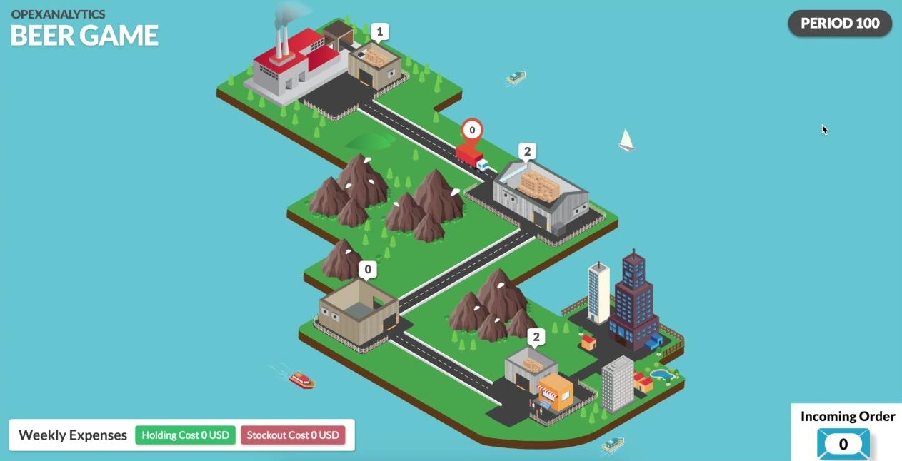
By the way, these screen shots and video come from a new, free, computerized version of the beer game developed by Opex Analytics. You can sign up to receive an e-mail when the game is released here.

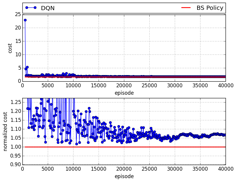
Numerical Results

The figures below plot the total cost of the four players for two cases: (1) when all four players use a base-stock policy, which is optimal for this setting and therefore provides a baseline (blue curve), and (2) when one of the players is replaced by the DQN agent (green curve). The x-axis indicates the number of episodes on which the DQN is trained. The upper subfigure indicates the total cost, while the lower subfigure indicates the normalized cost, in which the costs of the BS policy and the DQN are divided by BS policy's cost. The figures show that after a relatively small number of training episodes, the AI has learned to play nearly optimally.

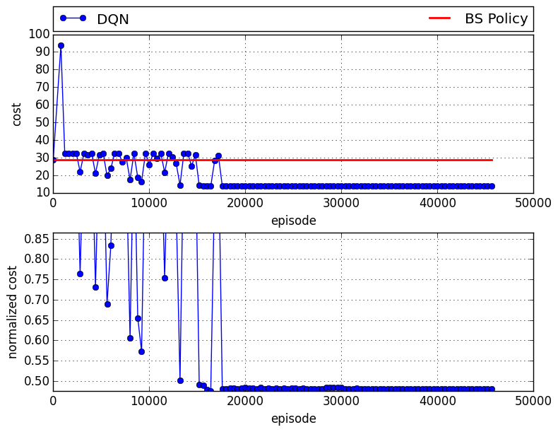
The following figure represents the case in which the DQN plays the retailer: 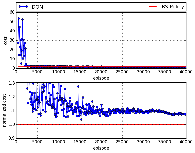After it has been sufficiently trained, there is roughly an 8% gap compared to the case in which all agents follow a base-stock policy.

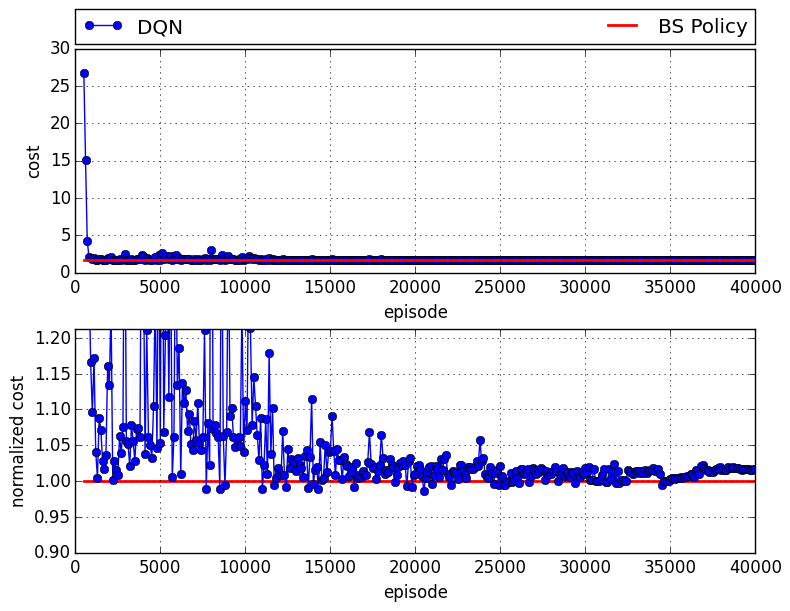
Here is the case in which the DQN plays the wholesaler: 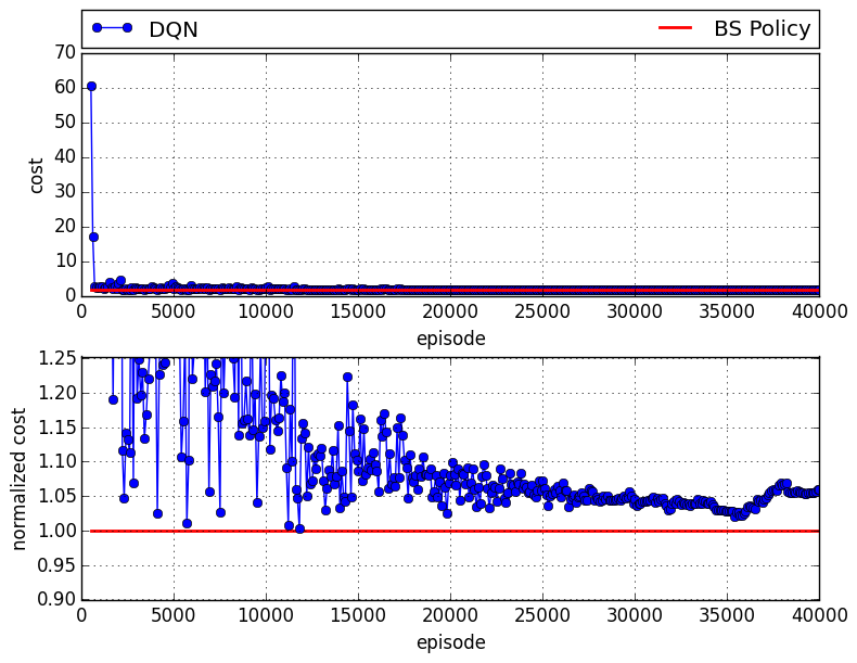There is an approximately 6% gap compared to the case in which all agents follow a base-stock policy.

When the DQN plays the distributor, there is a 7% gap:

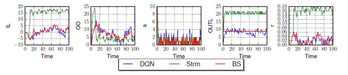
And finally, when the DQN plays the manufacturer:, there is about a 2% gap compared to the optimal solution: Also, the following figure shows the details of the inventory level (IL), on-order quantity (OO), order quantity (a), order up to level (OUTL), and reward (r) for the retailer when the retailer is played by the DQN. The BS policy and DQN have similar IL and OO trends, and as a result their rewards are also very close.

Play with Irrational Players

The agents who follow the BS are rational players. In order to see how well DQN works when it plays with irrational players, we tested the case that a DQN agent plays with three agents following the Sterman formula; see the following figure, which shows the corresponding results when the DQN plays the distributor. The DQN learns very well to play with other irrational players to minimize the total cost of the system, such that on average the DQN agents obtained $40\%$ smaller cost than the case in which the three Sterman players play with one BS policy. We get same results on other agents.

Transfer Learning

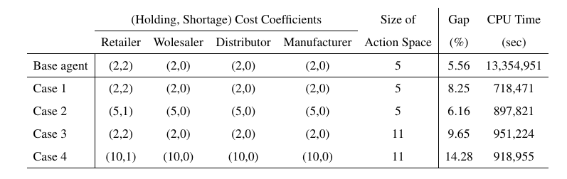
This procedure works well; however, for each new set of the number of actions, shortage and holding cost parameters we need to train a new policy, since they uniquely define the DQN loss function, and this is a time consuming procedure. To address this issue, we train a base agent with given cost parameters and action space, then transfer the acquired knowledge to the new agents, so that the obtained policy easily can be generalized to other agents. The following table shows the results of training new agents with different cost coefficients and different action spaces. As it is shown, the average gap is around 8.9\%, which shows the effectiveness of transfer learning approach. Additionally, the training times of each case are provided in the table. In order to get the base results, we did hyper-parameter tuning which resulted in total of 13,354,951 seconds training. However, following the transfer learning approach we do not need any hyper-parameter tuning, and on average we spent 891,117 seconds for training, which is 15 times faster.

Conclusion

The results above are surprising (at least to us) and impressive. They demonstrate that the DQN can learn to play close to the optimal solution, with just—and only just—some historical data, without any knowledge of how other the agents play, what their ordering policy is, etc.

These days, most companies have huge quantities of data about their supply chains. This research suggests that these data can be used by ML algorithms to make near-optimal decisions in a supply chain. In the future, we plan to adapt this approach to different supply chain structures with more complex networks and more agents. Stay tuned on this page for more results.

You can read our research paper, "A Deep Q-Network for the Beer Game with Partial Information," on arXiv. Visit the Opex Analytics beer game for the computerized version of the game. Also, the code of the paper is publicly available at github.